
After 13 years of anticipation, Grand Theft Auto VI (GTA VI) has finally arrived. The release represents one of the biggest entertainment events in recent history, but beyond the gameplay and commercial success of the franchise, it is worth appreciating what Rockstar Games has achieved as a piece of digital artwork.
The creation of an entire virtual world, complete with cities, transport networks, natural environments, architecture, weather systems and functioning ecosystems, is an extraordinary undertaking. From the geographical influences of real-world locations to the finer details of individual streets and buildings, there is a remarkable amount of creativity and technical expertise that goes into designing an open-world game of this scale.
Naturally, as GIS professionals, one of the things that interests us most is its geography.
Just how big is the GTA VI map, and what would it look like if we placed an equivalent area over some of the world's most recognisable cities?
Establishing the size of the GTA VI map
Before we could begin our mapping exercise, we needed to establish the size of the game world — something that turned out to be more complicated than expected.
Rockstar Games' fictional state of Leonida, inspired by Florida, has been widely reported to be approximately twice the size of the GTA V map. However, at the time of writing, an official measurement in square kilometres has not been established.
Various online sources and community mapping projects have produced significantly different estimates. Some of this variation can be attributed to the information available when the estimates were made, but an equally important consideration is the definition of the map itself.
Are we measuring the entire playable area, including the ocean? Are we measuring the terrestrial environment? What about rivers, lakes, canals and wetlands?
One particularly interesting set of measurements from the GTA mapping community demonstrated how much this definition could influence the result:
Land, excluding lakes, rivers and canals: 82.7 km²
Terrain above sea level: 87.2 km²
Land and coastal waters within 100 m of the shoreline: 113.4 km²
All modelled terrain, including ocean and river beds: 187.0 km²
More recent measurements of the community-reconstructed map have also produced land area estimates of approximately 82.6 km², while an earlier analysis produced an estimate of 83.2 km².
Given the consistency between these figures, we settled on a rounded estimate of 83 km² of land as the basis for our comparison.
While the actual map size may be refined as more information becomes available, this provided a reasonable starting point for our exercise.
Our mapping challenge
For a bit of fun, we set ourselves the challenge of mapping an equivalent land area around the centre of five major cities:
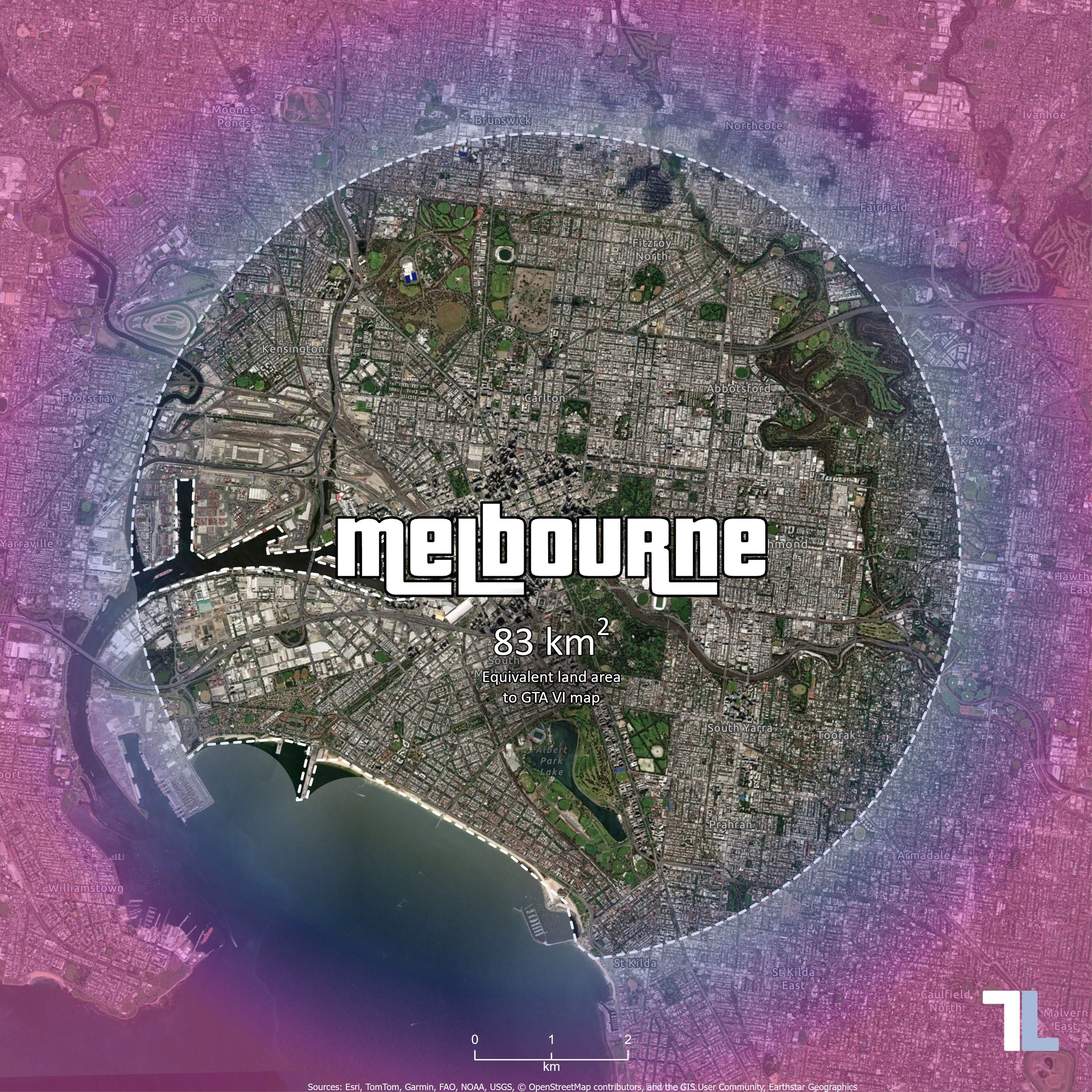
Melbourne, Australia
Miami, United States
New York, United States
London, United Kingdom
Beijing, China
Miami was an obvious inclusion, given its influence on the design of Vice City, while Melbourne provides a local comparison for our Australian audience. The remaining cities provide an interesting variety of urban landscapes and geographical characteristics.
Rather than attempting to recreate the shape of the GTA VI map, we decided to create circular boundaries extending outwards from each city centre.
On a completely terrestrial surface, a circle with an area of 83 km² would have a radius of approximately 5.14 km (you remember that equation from high school, right? RIGHT?).
However, most major cities have developed around waterways, and this introduced an interesting spatial problem. A circle centred on Melbourne would extend into Port Phillip Bay, while one centred on Manhattan would encompass substantial areas of the Hudson and East rivers.
If we simply applied a 5.14 km buffer to each city, we would end up with significantly different land areas.
Instead, we needed to increase the radius of each circle until the total area of land within it reached 83 km², regardless of how much water was also contained within the circle.
Developing the GIS workflow
While this could be achieved manually using a series of geoprocessing tools in ArcGIS Pro, it presented a good opportunity to develop a reusable Python script using ArcPy.
Before writing the script, there were several spatial considerations that needed to be worked through.
Selecting the city centres
The first step was to establish a central reference point for each city.
There is no definitive geographical centre for many major cities, and using the centroid of an administrative boundary would not necessarily produce a meaningful result. Instead, we selected recognisable landmarks that provide a reasonable representation of each city's centre.
Melbourne, Flinders Street Station
Miami, Bayfront Park
New York, Times Square
London, Charing Cross
Beijing, Tiananmen Square
The latitude and longitude coordinates of these locations could then be incorporated directly into the Python script, removing the need to manually digitise points for each city.
Establishing the land area
To distinguish between land and water, a global land polygon dataset was sourced from Esri's ArcGIS Living Atlas of the World and stored in a local geodatabase.
This provided a consistent spatial dataset that could be applied to all five cities, irrespective of national borders or administrative boundaries.
An important consideration was that the land did not need to be geographically connected to the city centre. In New York, for example, land on the New Jersey side of the Hudson River would need to contribute to the calculation in the same way as land on Manhattan.
The workflow therefore needed to accommodate islands, fragmented coastlines and multipart geometries.
Selecting appropriate map projections
Another important consideration was the coordinate system used to perform the analysis.
While latitude and longitude are convenient for identifying locations anywhere in the world, they are not particularly useful for creating accurate buffers measured in metres.
Similarly, a global projection such as Web Mercator, commonly used in online mapping applications, introduces substantial scale distortion that varies with latitude.
To minimise this distortion, we identified the appropriate local Universal Transverse Mercator (UTM) projection for each city.
Melbourne: WGS 84 / UTM Zone 55S EPSG 32755
Miami: WGS 84 / UTM Zone 17N EPSG 32617
New York: WGS 84 / UTM Zone 18N EPSG 32618
London: WGS 84 / UTM Zone 30N EPSG 32630
Beijing: WGS 84 / UTM Zone 50N EPSG 32650
By incorporating these coordinate systems into the script alongside the city centre coordinates, the necessary spatial transformations could be performed automatically.
Calculating the equivalent land area
The underlying GIS workflow was relatively straightforward. The more interesting challenge was determining the appropriate buffer radius without having to repeatedly run geoprocessing tools by hand.
The Python script was designed to perform the following operations for each city:
Create a point using the nominated latitude and longitude coordinates.
Project the point into the appropriate local UTM coordinate system.
Extract the surrounding land polygons and project them into the same coordinate system.
Dissolve the land polygons into a multipart geometry.
Create an initial circular buffer around the city centre.
Intersect the buffer with the land geometry, effectively removing any areas of water represented in the dataset.
Calculate the remaining land area.
Adjust the buffer radius and repeat the process until the land area reaches 83 km².
To make this process efficient, the script uses a binary search algorithm. Rather than incrementally increasing the radius by a fixed distance, the algorithm progressively narrows the range of possible radii until it converges on the target area.
If the land area is too small, the search radius is increased. If it is too large, the radius is reduced. Each iteration brings the result closer to the target.
A tolerance of 0.001 km² (1,000 m²) was applied to the calculation. While this level of computational precision is considerably greater than the accuracy of the estimated GTA VI map size, it ensures consistency between the five outputs.
The resulting feature classes included the full circular buffer, the land-only polygon and the city centre point, along with attributes recording the final radius and the respective areas of land and water.
The target area was also configured as a variable, meaning that the entire exercise could easily be repeated should a more accurate measurement of the GTA VI map become available.
From spatial analysis to cartography
With the spatial analysis complete, the next challenge was turning the results into something visually interesting.
Cartography is an interesting combination of science and art. While the spatial analysis determines what needs to be represented, the design of the map determines how effectively that information is communicated.
For this exercise, we wanted the maps to retain their geographical accuracy while incorporating some of the visual identity associated with Grand Theft Auto.
Map projections and scale
Individual maps were configured in ArcGIS Pro using the respective local UTM projection for each city.
Although it would have been simpler to use a single global coordinate system, doing so would have introduced varying degrees of distortion between cities at different latitudes.
All five maps were therefore produced at an identical scale of 1:48,000, using their respective local projections.
This was particularly important given the purpose of the exercise. We wanted readers to be able to move between the images and directly compare the extent of each area without differences in map scale influencing their perception of size.
Designing the layout
Square layouts were created to complement the predominantly circular nature of the boundaries and to provide a format suitable for social media platforms such as Instagram.
Aerial imagery was used as the basemap, allowing readers to recognise familiar buildings, parks, suburbs and infrastructure.
Rather than applying a solid colour to the land within the boundary, we chose to emphasise the surrounding area. This allowed the imagery inside the boundary to remain visible and encouraged readers to explore the geographical features contained within it.
A white dashed boundary was used to further distinguish the calculated land area from its surroundings.
Incorporating the GTA aesthetic
To give the maps a recognisable Grand Theft Auto appearance, we installed the Pricedown font, which is closely associated with the franchise's iconic logo.
This was used to display each city's name prominently in the centre of the map, with white lettering and a black outline.
We also wanted to incorporate the distinctive pink and purple colour palette associated with GTA VI's promotional artwork. Using colour picker tools, we sampled colours from artwork available online to establish a complementary colour scheme.
A square graphic was positioned over the entire layout and styled using a circular gradient fill. This allowed us to simulate a coloured vignette, gradually introducing the GTA-inspired colours towards the edges of the image while maintaining visibility of the underlying geography.
The combination of typography, colour, aerial imagery and spatial boundaries helped bring the technical analysis and creative design together.
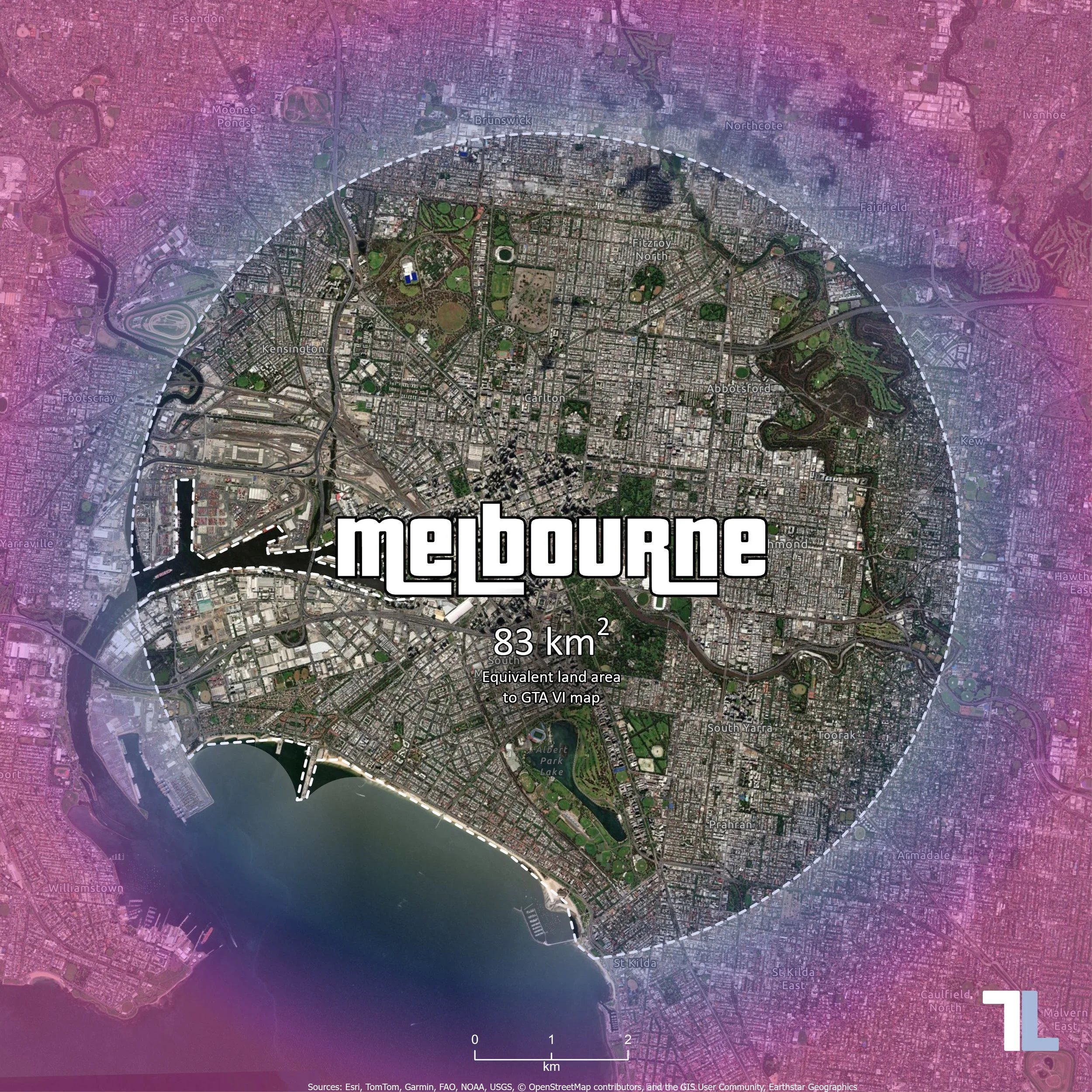
GTA VI map size comparison – 83 km² of land in Melbourne, Australia.
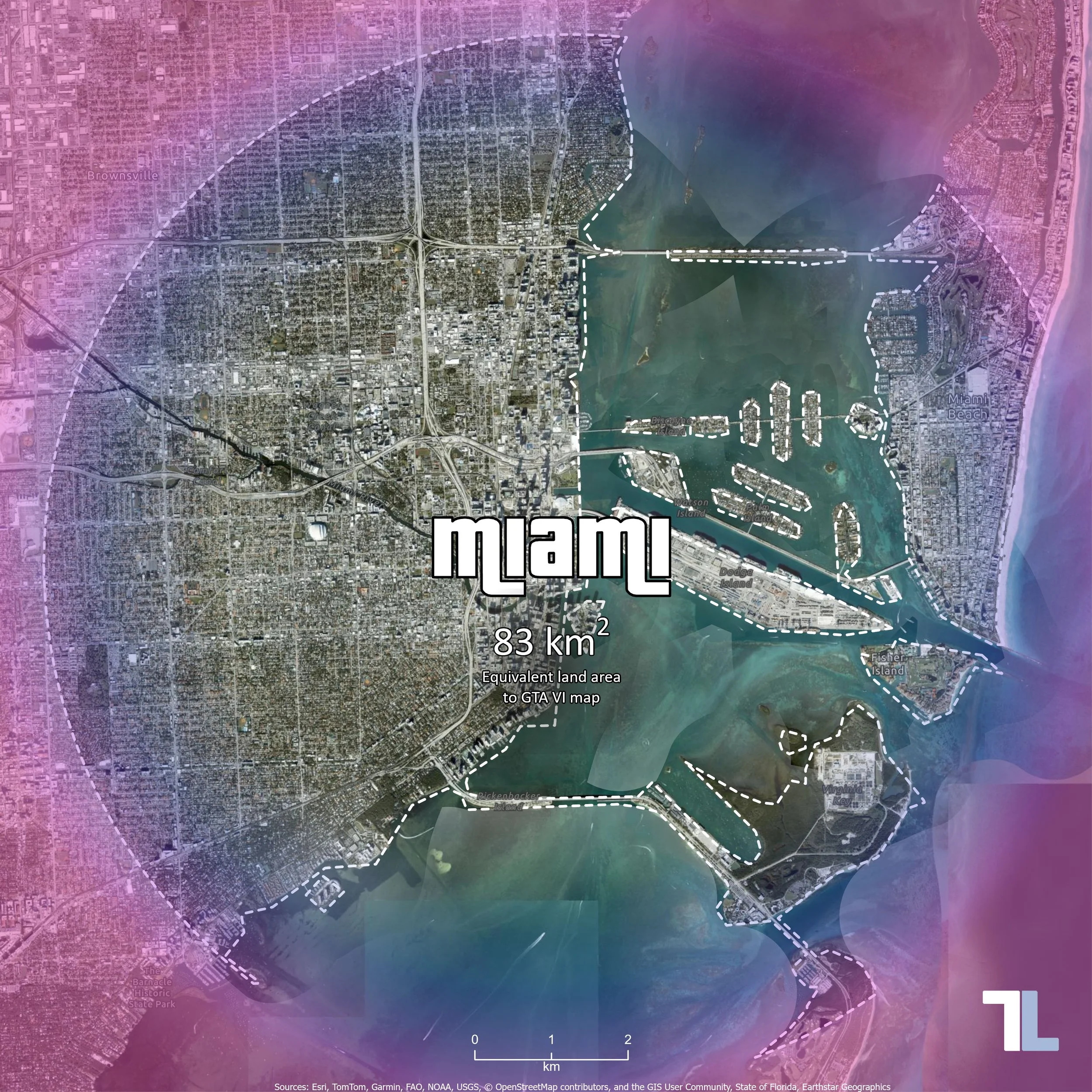
GTA VI map size comparison – 83 km² of land in Miami, USA.
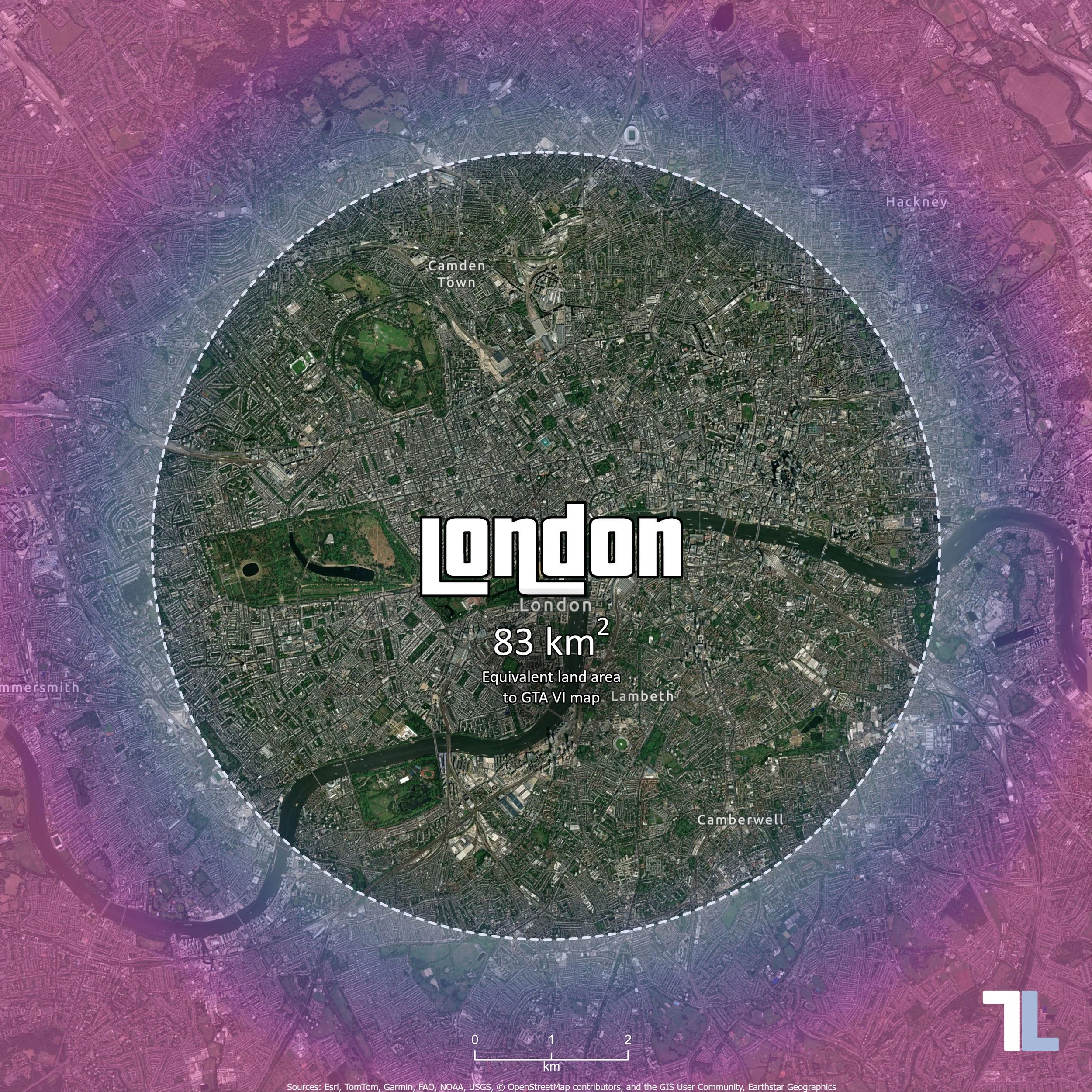
GTA VI map size comparison – 83 km² of land in London, UK.
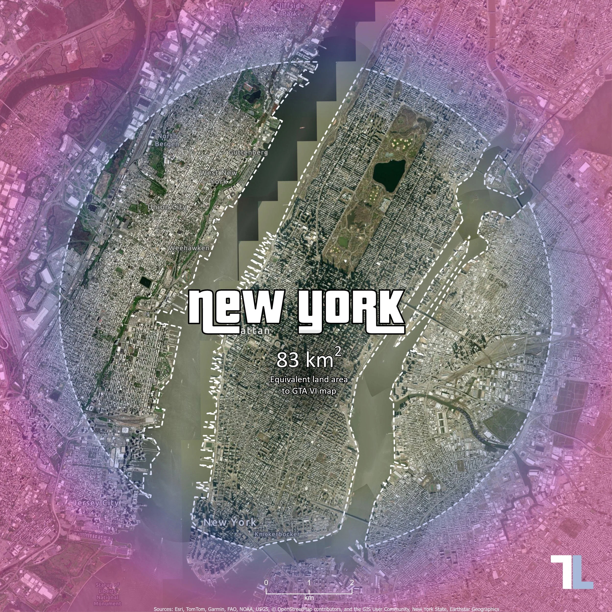
GTA VI map size comparison – 83 km² of land in New York, USA.
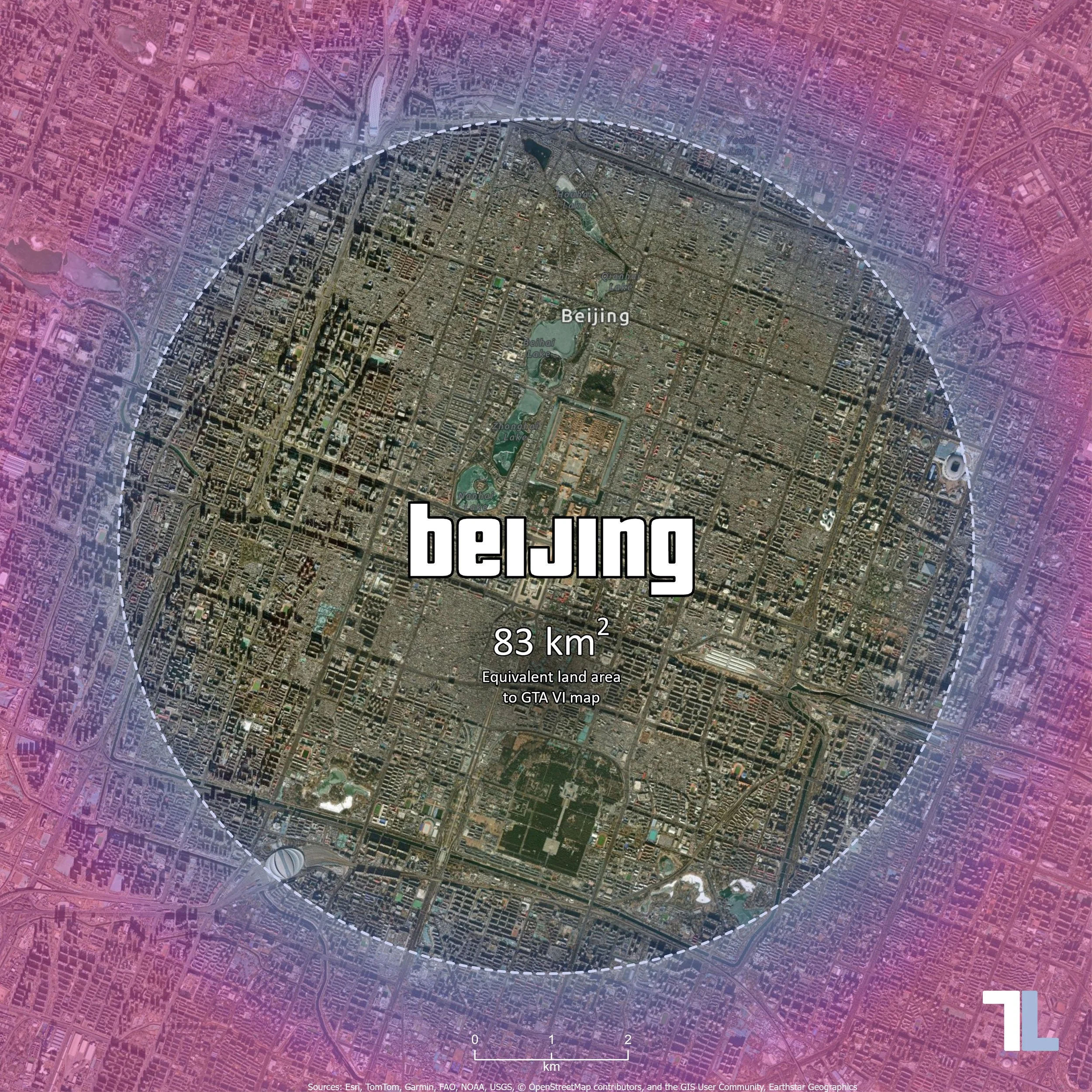
GTA VI map size comparison – 83 km² of land in Beijing, China.
Five cities, five different geographies, and 83 km² of land in each.
From the fragmented urban landscape of New York to the inland geography of Beijing, each map provides a different perspective on the scale of the GTA VI world.
The exercise is also a reminder of how much geography can influence something as seemingly simple as drawing a circle of a predetermined area.
At TerraLab, much of our work involves applying GIS to environmental management, infrastructure and real-world decision-making. But occasionally, it is just as rewarding to use the same tools and techniques to explore something completely different.
And what better excuse than the release of one of the most ambitious virtual worlds ever created?
Note: The GTA VI land area used in this exercise is based on community map estimates available in November 2026, rather than an official area measurement published by Rockstar Games.